
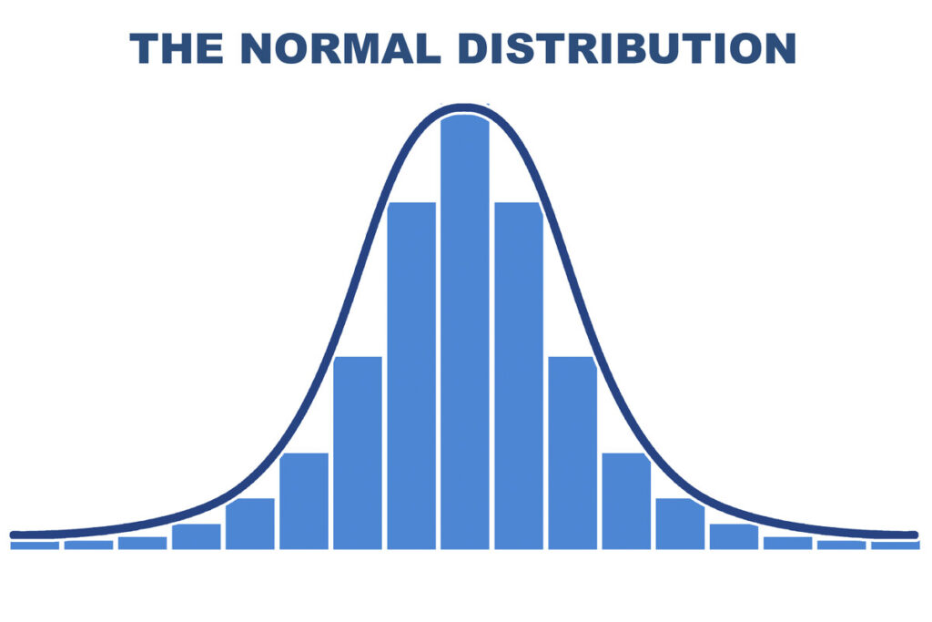
The bell curve shape that everyone associates with the normal distribution is not actually unique to it at all.
The normal distribution, often called the Gaussian distribution, shows up so often across statistics and science that people tend to assume its iconic shape belongs to it exclusively. It does not, and that is only the first surprise hiding inside this famous curve.
A shape defined by just two numbers
The normal distribution is a continuous probability distribution fully described by only two values: its mean and its variance. Its most famous property is the so called 68-95-99.7 rule, which states that about 68 percent of values fall within one standard deviation of the mean, 95 percent fall within two, and 99.7 percent fall within three.
Mathematically, it is one of a kind in a specific way: it is the only distribution where every statistical measure beyond the mean and variance equals exactly zero. It also carries the maximum possible entropy among all distributions sharing a given mean and variance, meaning it represents the least structured, most naturally spread out shape mathematically possible under those constraints.
The bell shape that several other distributions also share
Despite its nickname, the bell curve, plenty of other distributions share that same general shape without being normal distributions at all. The Cauchy distribution, the Student’s t distribution, and the logistic distribution all produce visually similar bell shaped curves, yet each behaves quite differently under the surface, particularly in how likely extreme values are to occur.
Statistician Roy C. Geary demonstrated something equally surprising: assuming a finite mean and variance, the normal distribution is the only one where the mean and variance calculated from independent observations remain fully independent of each other, a mathematical property unique to this single distribution.
Gauss did not start with today’s formula
Carl Friedrich Gauss originally defined the standard normal distribution using a formula with a variance of one half, quite different from the version universally used today. His work in 1809 applied the distribution directly to the theory of measurement errors in astronomy, a field demanding extreme precision.
Long before Gauss, in the early 18th century, Abraham de Moivre had already laid down the earliest rigorous mathematical groundwork for the distribution. Pierre Simon Laplace later connected it firmly to the central limit theorem during the 19th century, explaining why the normal distribution appears so often regardless of how the underlying data started out.
A curve that cannot handle everything thrown at it
It would be a mistake to assume the normal distribution fits every kind of data. It struggles badly with variables that are strictly positive or heavily skewed, things like a person’s weight or a stock’s price, which are far better modeled using distributions like the log normal or the Pareto distribution instead.
There is also a purely technical headache buried inside the curve. The error function needed to calculate its cumulative probability cannot be written using ordinary elementary functions at all, which is why mathematicians have had to develop an entire toolkit of numerical approximations just to work with it in practice.
Statistician Stephen Stigler even proposed an alternative version of the formula built around precision, the inverse of the standard deviation, simplifying calculations that the traditional version makes needlessly complicated. Two centuries after Gauss, the curve everyone thinks they understand is still being quietly refined.